Under The Hood: Scale Function Calculation In R Programming- Data Standardization As Part Of Distance Matrix Calculations In K Means Clustering

In the original blog post on website content segmentation via k means clustering in r programming, there were several statistical concepts that I felt required separate posts. In this particular blog, I’ll cover the scale() function and why that’s an important step.

The original dataset that I used for the K means clustering example was this website’s pages & metrics for them. Thinking about the metrics I included, I have pageviews [that had a range from a few hundred to a few K], bounce rate, entrance rate etc. Now, with all features put together for the dataset, if you wanted to create a distance matrix, you would need some way of standardizing the units.

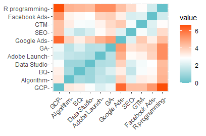
Example Distance Matrix from the k means clustering blog post here: https://analyticslog.com/blog/2021/2/20/google-analytics-content-segmentation-via-k-means-clustering-in-r-programming

The key in distance matrix is the distance between two data points that captures the variability in data. In the original blog post, Euclidian distance was used on the dataset across the different variables and then a weighted average was applied to measure the distance. Ok, now that we have some background, let’s start with the scale function.

I have put up a public Google sheet that contains the data used in k means clustering and will be used in this blog post as well. Link to data: https://docs.google.com/spreadsheets/d/1W8tzRMV0hHpa1xpVgRA0iqwKEI9-JPEuSWUCen1Ehqg/edit#gid=0

Let’s start with checking the scale function that’s the last step before creating a distance matrix.

In above code, we had loaded the dataset, tidyverse library, removed string values from the dataset as scale function requires it and then used scale() function.

Let’s pick a column, br [bounce rate]. After running the scale function, the column values show as above.

How are scaled values calculated for a column?

The individual value minus the mean of the column, divided by the standard deviation of the column.

(Xi - X bar)/SD(X)

Let’s work it out backwards to see how was it calculated for the column.
Step 1 - Let’s quickly check on the mean and SD for the ‘br’ column.

Let’s use select and mutate together to select the ‘br’ column and then add two new columns to show the mean of ‘br’ column and sd of ‘br’ column.

We’re on track here. The two additional columns show the same values for mean and standard deviation as expected. Let’s run another dplyr mutate function to complete the scaling part. Remember from earlier, it’s the individual value - mean divided by standard deviation.

There’s your last column, br_scaled, which has the exact values that you would get from scale() function directly. This was done on the original dataset and was available in data_scaled dataframe. Check below, the values match.

And that’s how this function was done across all of the variables to scale them between -1 and 1. In upcoming blog posts, I plan to cover other aspects such as Euclidian distance, PCA details and Elbow method. Full code below.